{
"cells": [
{
"cell_type": "markdown",
"metadata": {},
"source": [
"# Exercise IV: Logistic Regression"
]
},
{
"cell_type": "markdown",
"metadata": {},
"source": [
"> In statistics, the logistic model (or logit model) is used to model the probability of a certain class or event existing such as pass/fail, win/lose, alive/dead or healthy/sick. This can be extended to model several classes of events such as determining whether an image contains a cat, dog, lion, etc. Each object being detected in the image would be assigned a probability between 0 and 1, with a sum of one. [*Wikipedia*](https://en.wikipedia.org/wiki/Logistic_regression)"
]
},
{
"cell_type": "markdown",
"metadata": {},
"source": [
"In this exercise we will reproduce the bank defaults example used in chapter IV of the ISLR, as adapted from the [ISLR-python](https://github.com/JWarmenhoven/ISLR-python) repository."
]
},
{
"cell_type": "markdown",
"metadata": {},
"source": [
"## Setup"
]
},
{
"cell_type": "code",
"execution_count": 2,
"metadata": {
"tags": [
"hide-input"
]
},
"outputs": [],
"source": [
"import warnings\n",
"warnings.simplefilter(\"ignore\")"
]
},
{
"cell_type": "code",
"execution_count": 3,
"metadata": {},
"outputs": [],
"source": [
"import pandas as pd\n",
"\n",
"URL = \"https://github.com/JWarmenhoven/ISLR-python/raw/master/Notebooks/Data/Default.xlsx\"\n",
"df = pd.read_excel(URL, index_col=0, true_values=[\"Yes\"], false_values=[\"No\"])"
]
},
{
"cell_type": "code",
"execution_count": 4,
"metadata": {},
"outputs": [
{
"data": {
"text/html": [
"\n",
"\n",
" \n",
" \n",
" \n",
" default \n",
" student \n",
" balance \n",
" income \n",
" \n",
" \n",
" \n",
" \n",
" 965 \n",
" False \n",
" False \n",
" 0.000000 \n",
" 34305.918682 \n",
" \n",
" \n",
" 8655 \n",
" False \n",
" True \n",
" 17.609578 \n",
" 13739.754603 \n",
" \n",
" \n",
" 3649 \n",
" False \n",
" False \n",
" 370.033288 \n",
" 44507.211314 \n",
" \n",
" \n",
" 8672 \n",
" False \n",
" False \n",
" 761.187659 \n",
" 54681.828390 \n",
" \n",
" \n",
" 2605 \n",
" True \n",
" False \n",
" 1789.093391 \n",
" 48331.126858 \n",
" \n",
" \n",
" 7887 \n",
" False \n",
" True \n",
" 618.119217 \n",
" 24698.827238 \n",
" \n",
" \n",
" 1027 \n",
" False \n",
" False \n",
" 96.641839 \n",
" 44556.219419 \n",
" \n",
" \n",
" 3389 \n",
" False \n",
" False \n",
" 527.983482 \n",
" 39950.958521 \n",
" \n",
" \n",
" 8522 \n",
" False \n",
" False \n",
" 887.201436 \n",
" 41641.453572 \n",
" \n",
" \n",
" 1616 \n",
" False \n",
" False \n",
" 866.174669 \n",
" 41365.456380 \n",
" \n",
" \n",
" 6008 \n",
" False \n",
" True \n",
" 344.154112 \n",
" 20439.688108 \n",
" \n",
" \n",
" 6896 \n",
" False \n",
" False \n",
" 719.938044 \n",
" 31031.219396 \n",
" \n",
" \n",
" 2834 \n",
" False \n",
" False \n",
" 1820.325490 \n",
" 31309.998484 \n",
" \n",
" \n",
" 3974 \n",
" False \n",
" False \n",
" 615.465388 \n",
" 25865.180619 \n",
" \n",
" \n",
" 2154 \n",
" False \n",
" False \n",
" 1194.597579 \n",
" 38222.506106 \n",
" \n",
" \n",
"
\n"
],
"text/plain": [
""
]
},
"execution_count": 4,
"metadata": {},
"output_type": "execute_result"
}
],
"source": [
"def color_booleans(value: bool) -> str:\n",
" color = \"green\" if value else \"red\"\n",
" return f\"color: {color}\"\n",
"\n",
"BOOLEAN_COLUMNS = [\"default\", \"student\"]\n",
"\n",
"df.sample(15).style.text_gradient(cmap=\"Blues\").applymap(color_booleans, subset=BOOLEAN_COLUMNS)"
]
},
{
"cell_type": "markdown",
"metadata": {},
"source": [
"### Feature Scaling"
]
},
{
"cell_type": "code",
"execution_count": 5,
"metadata": {},
"outputs": [],
"source": [
"import numpy as np\n",
"from sklearn.preprocessing import StandardScaler\n",
"\n",
"numeric_features = df.select_dtypes(np.float)\n",
"scaler = StandardScaler()\n",
"df.loc[:, numeric_features.columns] = scaler.fit_transform(df.loc[:, numeric_features.columns])"
]
},
{
"cell_type": "markdown",
"metadata": {},
"source": [
"## Raw inspection"
]
},
{
"cell_type": "code",
"execution_count": 6,
"metadata": {},
"outputs": [
{
"name": "stdout",
"output_type": "stream",
"text": [
"\n",
"Int64Index: 10000 entries, 1 to 10000\n",
"Data columns (total 4 columns):\n",
" # Column Non-Null Count Dtype \n",
"--- ------ -------------- ----- \n",
" 0 default 10000 non-null bool \n",
" 1 student 10000 non-null bool \n",
" 2 balance 10000 non-null float64\n",
" 3 income 10000 non-null float64\n",
"dtypes: bool(2), float64(2)\n",
"memory usage: 253.9 KB\n"
]
}
],
"source": [
"df.info()"
]
},
{
"cell_type": "code",
"execution_count": 7,
"metadata": {},
"outputs": [
{
"data": {
"text/html": [
"\n",
"\n",
"
\n",
" \n",
" \n",
" balance \n",
" income \n",
" \n",
" \n",
" \n",
" \n",
" count \n",
" 10000 \n",
" 10000 \n",
" \n",
" \n",
" mean \n",
" -1.25056e-16 \n",
" -1.93623e-16 \n",
" \n",
" \n",
" std \n",
" 1.00005 \n",
" 1.00005 \n",
" \n",
" \n",
" min \n",
" -1.72708 \n",
" -2.45539 \n",
" \n",
" \n",
" 25% \n",
" -0.731136 \n",
" -0.913058 \n",
" \n",
" \n",
" 50% \n",
" -0.0242674 \n",
" 0.0776593 \n",
" \n",
" \n",
" 75% \n",
" 0.684184 \n",
" 0.771653 \n",
" \n",
" \n",
" max \n",
" 3.76056 \n",
" 3.0022 \n",
" \n",
" \n",
"
\n",
"
\u001b[0m in \u001b[0;36m\u001b[0;34m\u001b[0m\n\u001b[1;32m 4\u001b[0m \u001b[0mpredictions_manual\u001b[0m \u001b[0;34m=\u001b[0m \u001b[0mdefault_probability\u001b[0m\u001b[0;34m.\u001b[0m\u001b[0margmax\u001b[0m\u001b[0;34m(\u001b[0m\u001b[0maxis\u001b[0m\u001b[0;34m=\u001b[0m\u001b[0;36m1\u001b[0m\u001b[0;34m)\u001b[0m\u001b[0;34m\u001b[0m\u001b[0;34m\u001b[0m\u001b[0m\n\u001b[1;32m 5\u001b[0m \u001b[0;34m\u001b[0m\u001b[0m\n\u001b[0;32m----> 6\u001b[0;31m \u001b[0mnp\u001b[0m\u001b[0;34m.\u001b[0m\u001b[0marray_equal\u001b[0m\u001b[0;34m(\u001b[0m\u001b[0mpredictions\u001b[0m\u001b[0;34m,\u001b[0m \u001b[0mpredictions_manual\u001b[0m\u001b[0;34m)\u001b[0m\u001b[0;34m\u001b[0m\u001b[0;34m\u001b[0m\u001b[0m\n\u001b[0m",
"\u001b[0;31mNameError\u001b[0m: name 'np' is not defined"
]
}
],
"source": [
"predictions = sk_model.predict(X_test)\n",
"\n",
"# Manually returning the index of the maximal value\n",
"predictions_manual = default_probability.argmax(axis=1)\n",
"\n",
"np.array_equal(predictions, predictions_manual)"
]
},
{
"cell_type": "markdown",
"metadata": {},
"source": [
"### `statsmodels`"
]
},
{
"cell_type": "code",
"execution_count": 45,
"metadata": {},
"outputs": [
{
"name": "stdout",
"output_type": "stream",
"text": [
"Optimization terminated successfully.\n",
" Current function value: 0.078577\n",
" Iterations 10\n"
]
}
],
"source": [
"sm_estimation = sm_model.fit()"
]
},
{
"cell_type": "markdown",
"metadata": {},
"source": [
"## Model Evaluation"
]
},
{
"cell_type": "markdown",
"metadata": {},
"source": [
"### `sklearn`"
]
},
{
"cell_type": "code",
"execution_count": 39,
"metadata": {},
"outputs": [
{
"name": "stdout",
"output_type": "stream",
"text": [
"Intercept: [-10.55992039]\n",
"Coefficients: [[ 5.61993716e-03 -1.86000486e-06 -6.21154719e-01]]\n"
]
}
],
"source": [
"print(f\"Intercept: {sk_model.intercept_}\")\n",
"print(f\"Coefficients: {sk_model.coef_}\")"
]
},
{
"cell_type": "markdown",
"metadata": {},
"source": [
"#### Confusion Matrix"
]
},
{
"cell_type": "markdown",
"metadata": {},
"source": [
"##### Calculation"
]
},
{
"cell_type": "code",
"execution_count": 15,
"metadata": {},
"outputs": [
{
"name": "stdout",
"output_type": "stream",
"text": [
"[[1920 6]\n",
" [ 51 23]]\n"
]
}
],
"source": [
"from sklearn.metrics import confusion_matrix\n",
"\n",
"confusion_matrix_ = confusion_matrix(y_test, predictions)\n",
"print(confusion_matrix_)"
]
},
{
"cell_type": "markdown",
"metadata": {},
"source": [
"##### Visualization"
]
},
{
"cell_type": "code",
"execution_count": 16,
"metadata": {},
"outputs": [
{
"data": {
"image/png": "iVBORw0KGgoAAAANSUhEUgAAATUAAAEWCAYAAAAHJwCcAAAAOXRFWHRTb2Z0d2FyZQBNYXRwbG90bGliIHZlcnNpb24zLjMuMywgaHR0cHM6Ly9tYXRwbG90bGliLm9yZy/Il7ecAAAACXBIWXMAAAsTAAALEwEAmpwYAAAdR0lEQVR4nO3de5xd4/328c81kyM5yAmRg6gGjVNoJEKFopWgVFXrUEX1p+pQpdqfVh+UHn6tp7R9nqCUqmgdUqUhaaK0ETwOGUFIFHkhckBOCIJkZr7PH3tN7IzJzF6TvWfvWXO9vfare61173t9d8LVe617rbUVEZiZZUVVuQswMysmh5qZZYpDzcwyxaFmZpniUDOzTHGomVmmONQyRlJ3SXdLelvS5E3o5wRJ9xaztnKQ9A9JJ5W7Dms7DrUykXS8pBpJ70p6LfmP7zNF6PrLwFZAv4g4prWdRMSfI+LzRahnA5IOkBSS7my0fvdk/cwC+7lE0s0ttYuICRHxp1aWa+2QQ60MJJ0H/Ab4ObkAGgpcBRxZhO63BV6IiNoi9FUqy4GxkvrlrTsJeKFYO1CO//3uiCLCrzZ8Ab2Bd4FjmmnTlVzoLU1evwG6JtsOABYD3wOWAa8BpyTbfgKsBdYl+zgVuAS4Oa/vYUAAnZLlk4GXgHeAl4ET8tY/lPe5fYDZwNvJ/+6Tt20mcBnwcNLPvUD/jXy3hvqvAc5M1lUDS4CLgJl5bX8LLAJWA08A+yXrxzf6nk/n1fGzpI73gU8m676ZbL8auCOv/18C9wMq978XfhXv5f8na3tjgW7Anc20uRDYGxgJ7A6MBn6ct31rcuE4iFxwTZTUJyIuJjf6uy0iekTE9c0VImlz4HfAhIjoSS64nmqiXV9gatK2H3AFMLXRSOt44BRgS6ALcH5z+wZuAr6evD8EeJZcgOebTe7PoC/wF2CypG4RMb3R99w97zMnAqcBPYGFjfr7HrCrpJMl7Ufuz+6kSBLOssGh1vb6ASui+cPDE4BLI2JZRCwnNwI7MW/7umT7uoiYRm60smMr66kHdpHUPSJei4h5TbQ5DHgxIiZFRG1E3AL8B/hCXps/RsQLEfE+cDu5MNqoiPh/QF9JO5ILt5uaaHNzRKxM9vlrciPYlr7njRExL/nMukb9rSH353gFcDNwdkQsbqE/a2ccam1vJdBfUqdm2mzDhqOMhcm69X00CsU1QI+0hUTEe8BXgdOB1yRNlbRTAfU01DQob/n1VtQzCTgL+CxNjFwlnS/puWQm9y1yo9P+LfS5qLmNEfEYucNtkQtfyxiHWtt7BPgQ+GIzbZaSO+HfYCgfPzQr1HvAZnnLW+dvjIgZEfE5YCC50dd1BdTTUNOSVtbUYBJwBjAtGUWtlxwe/gD4CtAnIrYgdz5PDaVvpM9mDyUlnUluxLc06d8yxqHWxiLibXInxCdK+qKkzSR1ljRB0q+SZrcAP5Y0QFL/pH2Lly9sxFPAOElDJfUGftiwQdJWko5Mzq19SO4wtr6JPqYBOySXoXSS9FVgBHBPK2sCICJeBvYndw6xsZ5ALbmZ0k6SLgJ65W1/AxiWZoZT0g7AT4GvkTsM/YGkka2r3iqVQ60MkvND55E7+b+c3CHTWcBdSZOfAjXAXOAZYE6yrjX7+idwW9LXE2wYRFVJHUuBVeQC5ttN9LESOJzcifaV5EY4h0fEitbU1KjvhyKiqVHoDGA6ucs8FgIfsOGhZcOFxSslzWlpP8nh/s3ALyPi6Yh4EfgRMElS1035DlZZ5IkfM8sSj9TMLFMcamaWKQ41M8sUh5qZZUpzF4C2OXWpCrpVVEnWgj132KXcJVgKC195lRUrVqjllhun/t2CtU1d+dOEd9bNiIjxm7K/tCorQbp1gjFblrsKS+Hh6Q+VuwRLYd8xRXi61dr6wv87vW9JS3eAFF1lhZqZtQ/apMFeSTnUzCwdAdUONTPLksrNNIeamaUlH36aWYaIir4YzKFmZul5pGZmmVK5meZQM7OUPPtpZpnjw08zy5TKzTSHmpmlJKCqclPNoWZm6VVupjnUzCwlCaor90I1h5qZpeeRmpllimc/zSxTKjfTHGpmlpJnP80scyo30xxqZtYKvk3KzDJDfp6amWVN5WaaQ83MWsEjNTPLlMq9ocChZmYp+ZIOM8sch5qZZYrPqZlZZgjPfppZlggVOFKLElfSFIeamaXmUDOzzBBQXeBEQX1pS2mSQ83M0lHhI7VycKiZWWoONTPLkMInCsrBoWZmqVVwpjnUzCwd4cNPM8sSQZUq9452h5qZpeaRmpllSgVnWiU/FcnMKpEQVSrs1WJf0nhJz0taIOmCJrYPlfRvSU9Kmivp0Jb6dKiZWWqSCnq10Ec1MBGYAIwAjpM0olGzHwO3R8QewLHAVS3V5sNPM0tHUFWc56mNBhZExEsAkm4FjgTm57UJoFfyvjewtKVOHWpmlkrKSzr6S6rJW742Iq5N3g8CFuVtWwyMafT5S4B7JZ0NbA4c3NIOHWpmllqKUFsREaM2YVfHATdGxK8ljQUmSdolIjZ6r7xDzcxSKtptUkuAIXnLg5N1+U4FxgNExCOSugH9gWUb69QTBWaWjoozUQDMBoZL2k5SF3ITAVMatXkVOAhA0qeAbsDy5jr1SM3MUivGQC0iaiWdBcwAqoEbImKepEuBmoiYAnwPuE7SueQmDU6OiGafPelQM7NUBFRVFecgLyKmAdMarbso7/18YN80fTrUzCy1Qi6sLReHmpmlI98m1WFdc+7PWXjrI9Rcc0+5S+lw7q2ZxW6nHsLOpxzM5bf9/mPbP1y7lq/9/Bx2PuVg9jvnyyx8ffH6bZffeg07n3Iwu516CP+seRCAD9Z+yGe+czSjv/0F9jztUC6b9Nv17a+eMomdTzmY7uN3YMXbq0r/5cpMFDZJUK6b3ksaai3d15V1k/75N4788anlLqPDqaur47sTf8Lff3odT147jckz7+G5hQs2aHPjjMn06dGbeX+8j7OPOpkLb7gcgOcWLmDyA1OZ8/tpTPnZHzhn4iXU1dXRtXMXpv/yJh6/+m4eu+rv3FvzII899xQAY0d8mmm/uJGhWw5q669aNirwn3IoWagVeF9Xpj38bA2r3nm73GV0OLOfn8v2A7dlu4FD6dK5C8fsfxj3PHLfBm3ueeR+Tjj4KAC+tN94Zj71CBHBPY/cxzH7H0bXLl0YtvUQth+4LbOfn4skenTfHIB1tbXU1tauH4mM/OQItt16cNt+yTLrqCO19fd1RcRaoOG+LrOSWrryDQYP2Hr98qD+W7Nk5RtNtBkIQKfqTvTavCcrV7/Jkrz1DZ9dmny2rq6OMWccwdBjx3Lgnvsyeqfd2+DbVKaqKhX0KkttJey7qfu6PjY+l3SapBpJNawrx68EmhWmurqax66awoKbZ1Hz/FzmvfJCuUsqCxXv4tuSKPtEQURcGxGjImIUnctejmXANv22YvHy19cvL1nxOoP6bdVEm9cAqK2rZfV779CvVx8G5a1v+Ow2jT67RY9e7L/7GO5NJhE6no47UVDIfV1mRTdqx11ZsPQVXnl9EWvXrWXyA1M5bO+DNmhz2N4H8uf77gTgbw9OZ//dxyKJw/Y+iMkPTOXDtWt55fVFLFj6CnvtuBvL31rFW++uBuD9Dz/g/jkPs+OQT7T5d6sUlRxqpbxObf19XeTC7Fjg+BLur+L86YIr2G+30fTv1YcFk2Zx2c2/408z/lrusjKvU3UnrjzjIr5w4anU1ddx0ue/zIhhw7n0pt+y5/BdOHzsQZw8/hi+8avvs/MpB9OnZ28m/fBKAEYMG87R4w5lj29NoFNVJ35z5sVUV1fz+qpl/Nev/5u6unrqo56jx03g0DGfBWDiXTdxxV+v441VK9jr20cwfq9xXH3uz8v5R1BylXydmlq4jWrTOs89evc3fHRf18+abd+rSzBmy5LVY8X3/vSOeV6pvdp3zGd4ombOJkVS96G9Y9j3Crtz6T/f/ccTm/joodRKekdBU/d1mVn751+TMrNMqeBMc6iZWVrlmwQohEPNzFJzqJlZZjRcfFupHGpmllq5boEqhEPNzNLzSM3MssMTBWaWJRX+5FuHmpmlkvIX2tucQ83MUnOomVmmePbTzLKjjI8VKoRDzcxS8Tk1M8sch5qZZYpDzcyyQ54oMLMMke8oMLOscaiZWaZUcKY51MwsJT9Pzcwyx6FmZlkhoNqzn2aWHZU9+1lV7gLMrJ0RVEkFvVrsShov6XlJCyRdsJE2X5E0X9I8SX9pqU+P1MwslWLd+ympGpgIfA5YDMyWNCUi5ue1GQ78ENg3It6UtGVL/XqkZmapVRX4asFoYEFEvBQRa4FbgSMbtfkvYGJEvAkQEcta6nSjIzVJ/weIjW2PiO+0XLOZZU1uoqDg8VB/STV5y9dGxLXJ+0HAorxti4ExjT6/A4Ckh4Fq4JKImN7cDps7/KxpZpuZdViFnS9LrIiIUZuws07AcOAAYDAwS9KuEfFWcx9oUkT8KX9Z0mYRsWYTijOzLCjexbdLgCF5y4OTdfkWA49FxDrgZUkvkAu52RvrtMUxpKSxkuYD/0mWd5d0VcrizSwjRNHOqc0GhkvaTlIX4FhgSqM2d5EbpSGpP7nD0Zea67SQA+PfAIcAKwEi4mlgXAGfM7OMKsYlHRFRC5wFzACeA26PiHmSLpV0RNJsBrAyGVj9G/h+RKxsrt+CLumIiEWNhpt1hXzOzLKpWBffRsQ0YFqjdRflvQ/gvORVkEJCbZGkfYCQ1Bk4h1yqmlkHJKC6gu8oKCTUTgd+S276dSm54eCZpSzKzCpZqtnPNtdiqEXECuCENqjFzNoBJbdJVapCZj8/IeluScslLZP0d0mfaIvizKwyKfntz5Ze5VDI7OdfgNuBgcA2wGTgllIWZWaVrVg3tJektgLabBYRkyKiNnndDHQrdWFmVpmU4lUOzd372Td5+4/kkSC3krsX9Ks0moI1s45EdCr83s8219xEwRPkQqwhcL+Vty3IPQ7EzDoYtdffKIiI7dqyEDNrPyp59rOgOwok7QKMIO9cWkTcVKqizKyyVW6kFRBqki4md0PpCHLn0iYADwEONbMOSLT/kdqXgd2BJyPiFElbATeXtiwzq1xK85DINldIqL0fEfWSaiX1Apax4TOQzKwDaXj0UKUqJNRqJG0BXEduRvRd4JFSFmVmFay9zn42iIgzkrfXSJoO9IqIuaUty8wqWbs8pyZpz+a2RcSc0pRkZpWsPU8U/LqZbQEcWORa6N53c3b6yl7F7tZK6P4lM8pdgqWweu3qovTTLg8/I+KzbVmImbUXolqVO1XgX2g3s1Qq/XlqDjUzS00VfE+BQ83MUqvkc2qFPPlWkr4m6aJkeaik0aUvzcwqkSjsAZGV/JDIq4CxwHHJ8jvAxJJVZGYVT1QV9CqHQg4/x0TEnpKeBIiIN5NfUzazDqq93/u5TlI1uWvTkDQAqC9pVWZWsZT8U6kKCbXfAXcCW0r6Gbmndvy4pFWZWeVq75d0RMSfJT0BHETuDokvRoR/od2sA6vk2c9CHhI5FFgD3J2/LiJeLWVhZlaZco8eat/n1Kby0Q+wdAO2A54Hdi5hXWZWsURVe54oiIhd85eTp3ecsZHmZtYBVLXziYINRMQcSWNKUYyZVT7R/s+pnZe3WAXsCSwtWUVmVtna++wn0DPvfS25c2x3lKYcM6t87fg6teSi254RcX4b1WNmFS735Nt2OFEgqVNE1Eraty0LMrPKV8mh1lxljyf/+5SkKZJOlPSlhldbFGdmlah4T+mQNF7S85IWSLqgmXZHSwpJo1rqs5Bzat2AleR+k6DherUA/lbAZ80sY0RxHhKZnN6aCHwOWAzMljQlIuY3atcTOAd4rJB+mwu1LZOZz2f5KMwaRIrazSxjijT7ORpYEBEvAUi6FTgSmN+o3WXAL4HvF1RbM9uqgR7Jq2fe+4aXmXVEAqmqoBfQX1JN3uu0vJ4GAYvylhcn6z7aVe5i/yERMbXQ8pobqb0WEZcW2pGZdRSpLulYEREtngdrci+5VLwCODnN55oLtcq9EMXMykYU7SGRS4AhecuDk3UNegK7ADOTOxi2BqZIOiIiajbWaXOhdlDrazWzLCvSvZ+zgeGStiMXZscCxzdsjIi3gf4Ny5JmAuc3F2i52jYiIlZtYsFmlkEN934W8mpORNQCZwEzgOeA2yNinqRLJR3R2vr8E3lmlpIaJgE2WURMA6Y1WnfRRtoeUEifDjUzSy1Tjx4ys45NquzbpBxqZpZSy+fLysmhZmap+fDTzDIjN/vpw08zy4x2/JBIM7Om+JyamWWKZz/NLDNyP2bskZqZZUUBt0CVk0PNzFJTs49iLC+Hmpml5pGamWWGENWeKDCzLPF1amaWKT78NLPMyP1Eng8/zSwzfEmHmWWML741s8zwQyLNLHN8+GlmGSJPFJhZtlR5pJZNYwbtxnf3PpFqVXH3CzOZNPfuj7U5cLsxnDryaIJgwapXueSBiQCcMepY9hkyEoA/PnUX97/8aFuW3mE98cx8rr3lDuqjns/vN5ZjDv38BtunzXyIqf+aRVVVFd27duWsk45l6DYDWf3ue/ziqut58ZWFHLTvGL59wlfK9A3KL3dJRwcMNUk3AIcDyyJil1Ltp1yqJM4fezLnzPgFy95bxfVHXMaDr87hlbeWrG8zuNdWfH23Izh96iW8s3YNfbr1AmCfwSPZod8wTrrrR3Su7szECRfyyOKnWbPu/XJ9nQ6hrr6eq/88mZ9+70z69dmCcy+7nDEjd2XoNgPXtzlgzKc59IDPAPDYU8/wh9vu5NJzz6BL50587ajDWLjkNRYuWVqur1AxKvmcWikPjG8Expew/7Ia0X97Fq9+g6XvLKe2vo77XnqU/YZ+eoM2R+xwIHc890/eWbsGgDc/WA3AsC0G8dTr/6Eu6vmg9kMWvLmIvQfv1ubfoaN54aWFDNyyP1sP6E/nTp0YN/rTPPrkMxu02ax79/XvP/jww/XjkW5du7Lz8O3p0skHNyCqVFXQqxxK9jcUEbMkDStV/+U2YPO+vPHeyvXLy99bxYgB22/QZmjvrQG45rCLqVIV1z95B48tmcuCVa/yjT2+xC3PTqNbpy7sOXDEBiM8K42Vb73FgL591i/377MFz7/8ysfa3fOvWdx177+pra3lZ98/uw0rbB9yD4n0RMFGSToNOA2gc9/uLbRuX6pVzZDeW3HmtJ+y5eZ9uerQ/8WJd13A40uf4VMDPsHvD7+Etz5YzbPLXqSuvr7c5Vri8APHcfiB45j5aA233TOD8049sdwlVRZ13MPPgkTEtRExKiJGderZtdzlFGz5e6vYavN+65cHbN6X5Wve3KDNsjWreOjVOdRFHa+9u5xFq19jSK/c6O1PT/+dk//+I747438QYtHq19q0/o6o3xZbsHzVR39HK958i35bbLHR9uNG78mjT85tg8raGxX8TzmUPdTaq+dWvMTg3lszsMcAOlVVc/An9uahV5/YoM2shTXssfWnAOjdtQdDeg1kyTvLqJLo1bUHANv3GcIn+w7h8SXPfGwfVlw7bDeUpW8s5/XlK1hXW8usx59gzMhdN2iz5I1l69/PnjuPbbYc0NZltgtKHund0qscyn742V7VRT1XPHIjVx7y31SrintefICX31rCN/c4mv+seJmHFs3hsSVzGTNoV/581K+oj3omzv4Lqz98ly7Vnbn60IsAeG/d+/zkgaupCx9+llp1dTWnn3AMF115FfX1wec+szfbDhrIzXdNZfiwoYwZuSv33D+Lp597nurqanpsthnn5h16fuMHF7Pm/Q+oravl0Sef4bLzzthg5rSjqPRzaoqI0nQs3QIcAPQH3gAujojrm/vMZsP6xE4XHlCSeqw0Ljvk6+UuwVL47uHf58W5CzZpCDVi5E5x0303FNR2rwH7PhERozZlf2mVcvbzuFL1bWbl5F9oN7OMqeTZT4eamaXmkZqZZUolh1rlTmGYWUVSEW+TkjRe0vOSFki6oInt50maL2mupPslbdtSnw41M0utGBffSqoGJgITgBHAcZJGNGr2JDAqInYD/gr8qqXaHGpmlo6KdvHtaGBBRLwUEWuBW4Ej8xtExL8jYk2y+CgwuKVOHWpmllqKkVp/STV5r9PyuhkELMpbXpys25hTgX+0VJsnCswsFZHqko4Vxbj4VtLXgFHA/i21daiZWUpFu/h2CTAkb3lwsm7DvUkHAxcC+0fEhy116lAzs9SK9ADI2cBwSduRC7NjgePzG0jaA/g9MD4iln28i49zqJlZasUYqUVEraSzgBlANXBDRMyTdClQExFTgMuBHsDk5JD31Yg4orl+HWpmlkoxf3glIqYB0xqtuyjv/cFp+3SomVlK5XtWWiEcambWCg41M8sKFW2ioCQcamaWWiXf0O5QM7NU5HNqZpY1HqmZWaY41MwsU3z4aWaZ0fCQyErlUDOz1Hz4aWYZ41Azswyp3EhzqJlZK3iiwMwyxqFmZplRtCffloRDzcxSkSr78LNyLzYxM2sFj9TMLDUffppZpjjUzCxTfE7NzKyNeKRmZin5kg4zyxyHmpllhKjkSHOomVkrVPJEgUPNzFLzOTUzyxiHmpllRmX/RJ6vUzOzTPFIzcxSyc1+Vu5IzaFmZq3gUDOzDKmq4HNqDjUzS6myL791qJlZapUbaQ41M2uVyo01h5qZpVPhv1HgUDOzVCr9kg5FRLlrWE/ScmBhuesogf7AinIXYalk9e9s24gYsCkdSJpO7s+nECsiYvym7C+tigq1rJJUExGjyl2HFc5/Z+2Xb5Mys0xxqJlZpjjU2sa15S7AUvPfWTvlc2pmlikeqZlZpjjUzCxTHGolJGm8pOclLZB0QbnrsZZJukHSMknPlrsWax2HWolIqgYmAhOAEcBxkkaUtyorwI1Am14sasXlUCud0cCCiHgpItYCtwJHlrkma0FEzAJWlbsOaz2HWukMAhblLS9O1plZCTnUzCxTHGqlswQYkrc8OFlnZiXkUCud2cBwSdtJ6gIcC0wpc01mmedQK5GIqAXOAmYAzwG3R8S88lZlLZF0C/AIsKOkxZJOLXdNlo5vkzKzTPFIzcwyxaFmZpniUDOzTHGomVmmONTMLFMcau2IpDpJT0l6VtJkSZttQl83Svpy8v4Pzd1sL+kASfu0Yh+vSPrYrw5tbH2jNu+m3Nclks5PW6Nlj0OtfXk/IkZGxC7AWuD0/I2SWvU7rhHxzYiY30yTA4DUoWZWDg619utB4JPJKOpBSVOA+ZKqJV0uabakuZK+BaCc/5s83+0+YMuGjiTNlDQqeT9e0hxJT0u6X9IwcuF5bjJK3E/SAEl3JPuYLWnf5LP9JN0raZ6kP0DLv3gr6S5JTySfOa3RtiuT9fdLGpCs217S9OQzD0raqSh/mpYZ/oX2digZkU0Apier9gR2iYiXk2B4OyL2ktQVeFjSvcAewI7knu22FTAfuKFRvwOA64BxSV99I2KVpGuAdyPifyft/gJcGREPSRpK7q6JTwEXAw9FxKWSDgMKuRr/G8k+ugOzJd0RESuBzYGaiDhX0kVJ32eR+0GU0yPiRUljgKuAA1vxx2gZ5VBrX7pLeip5/yBwPbnDwscj4uVk/eeB3RrOlwG9geHAOOCWiKgDlkr6VxP97w3MaugrIjb2XLGDgRHS+oFYL0k9kn18KfnsVElvFvCdviPpqOT9kKTWlUA9cFuy/mbgb8k+9gEm5+27awH7sA7Eoda+vB8RI/NXJP9xv5e/Cjg7ImY0andoEeuoAvaOiA+aqKVgkg4gF5BjI2KNpJlAt400j2S/bzX+MzDL53Nq2TMD+LakzgCSdpC0OTAL+Gpyzm0g8NkmPvsoME7Sdsln+ybr3wF65rW7Fzi7YUHSyOTtLOD4ZN0EoE8LtfYG3kwCbSdyI8UGVUDDaPN4coe1q4GXJR2T7EOSdm9hH9bBONSy5w/kzpfNSX485PfkRuR3Ai8m224i9ySKDUTEcuA0cod6T/PR4d/dwFENEwXAd4BRyUTEfD6ahf0JuVCcR+4w9NUWap0OdJL0HPA/5EK1wXvA6OQ7HAhcmqw/ATg1qW8efkS6NeKndJhZpnikZmaZ4lAzs0xxqJlZpjjUzCxTHGpmlikONTPLFIeamWXK/we7Z388ggqf6wAAAABJRU5ErkJggg==\n",
"text/plain": [
""
]
},
"metadata": {
"needs_background": "light"
},
"output_type": "display_data"
}
],
"source": [
"from sklearn.metrics import plot_confusion_matrix\n",
"\n",
"disp = plot_confusion_matrix(sk_model,\n",
" X_test,\n",
" y_test,\n",
" cmap=plt.cm.Greens,\n",
" normalize=\"true\")\n",
"_ = disp.ax_.set_title(f\"Confusion Matrix\")"
]
},
{
"cell_type": "markdown",
"metadata": {},
"source": [
"#### Classification Report"
]
},
{
"cell_type": "code",
"execution_count": 17,
"metadata": {},
"outputs": [
{
"name": "stdout",
"output_type": "stream",
"text": [
" precision recall f1-score support\n",
"\n",
" 0 0.97 1.00 0.99 1926\n",
" 1 0.79 0.31 0.45 74\n",
"\n",
" accuracy 0.97 2000\n",
" macro avg 0.88 0.65 0.72 2000\n",
"weighted avg 0.97 0.97 0.97 2000\n",
"\n"
]
}
],
"source": [
"from sklearn.metrics import classification_report\n",
"\n",
"report = classification_report(y_test, predictions)\n",
"print(report)"
]
},
{
"cell_type": "markdown",
"metadata": {},
"source": [
"\n",
"*[Wikipedia](https://en.wikipedia.org/wiki/Precision_and_recall)*"
]
},
{
"cell_type": "markdown",
"metadata": {},
"source": [
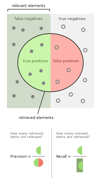
"##### Precision"
]
},
{
"cell_type": "markdown",
"metadata": {},
"source": [
""
]
},
{
"cell_type": "code",
"execution_count": 41,
"metadata": {},
"outputs": [
{
"data": {
"text/plain": [
"0.7931034482758621"
]
},
"execution_count": 41,
"metadata": {},
"output_type": "execute_result"
}
],
"source": [
"true_positive = confusion_matrix_[1, 1]\n",
"false_positive = confusion_matrix_[0, 1]\n",
"\n",
"true_positive / (true_positive + false_positive)"
]
},
{
"cell_type": "markdown",
"metadata": {},
"source": [
"##### Recall (Sensitivity)"
]
},
{
"cell_type": "markdown",
"metadata": {},
"source": [
""
]
},
{
"cell_type": "code",
"execution_count": 42,
"metadata": {},
"outputs": [
{
"data": {
"text/plain": [
"0.3108108108108108"
]
},
"execution_count": 42,
"metadata": {},
"output_type": "execute_result"
}
],
"source": [
"false_negative = confusion_matrix_[1, 0]\n",
"\n",
"true_positive / (true_positive + false_negative)"
]
},
{
"cell_type": "markdown",
"metadata": {},
"source": [
"##### Specificity"
]
},
{
"cell_type": "markdown",
"metadata": {},
"source": [
""
]
},
{
"cell_type": "code",
"execution_count": 43,
"metadata": {},
"outputs": [
{
"data": {
"text/plain": [
"0.9968847352024922"
]
},
"execution_count": 43,
"metadata": {},
"output_type": "execute_result"
}
],
"source": [
"true_negative = confusion_matrix_[0, 0]\n",
"\n",
"true_negative / (true_negative + false_positive)"
]
},
{
"cell_type": "markdown",
"metadata": {},
"source": [
"##### Accuracy Score"
]
},
{
"cell_type": "code",
"execution_count": 33,
"metadata": {},
"outputs": [
{
"data": {
"text/plain": [
"0.9715"
]
},
"execution_count": 33,
"metadata": {},
"output_type": "execute_result"
}
],
"source": [
"from sklearn.metrics import accuracy_score\n",
"\n",
"accuracy_score(y_test, predictions)"
]
},
{
"cell_type": "markdown",
"metadata": {},
"source": [
"or:"
]
},
{
"cell_type": "code",
"execution_count": 37,
"metadata": {},
"outputs": [
{
"data": {
"text/plain": [
"0.9715"
]
},
"execution_count": 37,
"metadata": {},
"output_type": "execute_result"
}
],
"source": [
"true_predictions = confusion_matrix_[0, 0] + confusion_matrix_[1, 1]\n",
"true_predictions / len(X_test)"
]
},
{
"cell_type": "markdown",
"metadata": {},
"source": [
"### `statsmodels`"
]
},
{
"cell_type": "markdown",
"metadata": {},
"source": [
"#### Confusion Matrix"
]
},
{
"cell_type": "code",
"execution_count": 18,
"metadata": {},
"outputs": [
{
"data": {
"text/plain": [
"array([[9627., 40.],\n",
" [ 228., 105.]])"
]
},
"execution_count": 18,
"metadata": {},
"output_type": "execute_result"
}
],
"source": [
"prediction_table = sm_estimation.pred_table()\n",
"prediction_table"
]
},
{
"cell_type": "code",
"execution_count": 19,
"metadata": {},
"outputs": [
{
"data": {
"text/plain": [
"array([[0.99586221, 0.00413779],\n",
" [0.68468468, 0.31531532]])"
]
},
"execution_count": 19,
"metadata": {},
"output_type": "execute_result"
}
],
"source": [
"row_sums = prediction_table.sum(axis=1, keepdims=True)\n",
"prediction_table / row_sums"
]
},
{
"cell_type": "markdown",
"metadata": {},
"source": [
"#### Regression Report"
]
},
{
"cell_type": "code",
"execution_count": 20,
"metadata": {},
"outputs": [
{
"data": {
"text/html": [
"\n",
"Logit Regression Results \n",
"\n",
" Dep. Variable: default No. Observations: 10000 \n",
" \n",
"\n",
" Model: Logit Df Residuals: 9996 \n",
" \n",
"\n",
" Method: MLE Df Model: 3 \n",
" \n",
"\n",
" Date: Wed, 25 Nov 2020 Pseudo R-squ.: 0.4619 \n",
" \n",
"\n",
" Time: 09:36:17 Log-Likelihood: -785.77 \n",
" \n",
"\n",
" converged: True LL-Null: -1460.3 \n",
" \n",
"\n",
" Covariance Type: nonrobust LLR p-value: 3.257e-292 \n",
" \n",
"
\n",
"\n",
"\n",
" coef std err z P>|z| [0.025 0.975] \n",
" \n",
"\n",
" Intercept -5.9752 0.194 -30.849 0.000 -6.355 -5.596 \n",
" \n",
"\n",
" balance 2.7747 0.112 24.737 0.000 2.555 2.995 \n",
" \n",
"\n",
" income 0.0405 0.109 0.370 0.712 -0.174 0.255 \n",
" \n",
"\n",
" student -0.6468 0.236 -2.738 0.006 -1.110 -0.184 \n",
" \n",
"
\n",
"\"\"\"\n",
" Logit Regression Results \n",
"==============================================================================\n",
"Dep. Variable: default No. Observations: 10000\n",
"Model: Logit Df Residuals: 9996\n",
"Method: MLE Df Model: 3\n",
"Date: Wed, 25 Nov 2020 Pseudo R-squ.: 0.4619\n",
"Time: 09:36:17 Log-Likelihood: -785.77\n",
"converged: True LL-Null: -1460.3\n",
"Covariance Type: nonrobust LLR p-value: 3.257e-292\n",
"==============================================================================\n",
" coef std err z P>|z| [0.025 0.975]\n",
"------------------------------------------------------------------------------\n",
"Intercept -5.9752 0.194 -30.849 0.000 -6.355 -5.596\n",
"balance 2.7747 0.112 24.737 0.000 2.555 2.995\n",
"income 0.0405 0.109 0.370 0.712 -0.174 0.255\n",
"student -0.6468 0.236 -2.738 0.006 -1.110 -0.184\n",
"==============================================================================\n",
"\n",
"Possibly complete quasi-separation: A fraction 0.15 of observations can be\n",
"perfectly predicted. This might indicate that there is complete\n",
"quasi-separation. In this case some parameters will not be identified.\n",
"\"\"\""
]
},
"execution_count": 20,
"metadata": {},
"output_type": "execute_result"
}
],
"source": [
"sm_estimation.summary()"
]
}
],
"metadata": {
"celltoolbar": "Tags",
"kernelspec": {
"display_name": "Python 3",
"language": "python",
"name": "python3"
},
"language_info": {
"codemirror_mode": {
"name": "ipython",
"version": 3
},
"file_extension": ".py",
"mimetype": "text/x-python",
"name": "python",
"nbconvert_exporter": "python",
"pygments_lexer": "ipython3",
"version": "3.8.10"
}
},
"nbformat": 4,
"nbformat_minor": 4
}