Exercise III: Linear Regression
In statistics, linear regression is a linear approach to modeling the relationship between a scalar response (or dependent variable) and one or more explanatory variables (or independent variables). Wikipedia
Using linear regression with Python is as easy as running:
>>> from sklearn.linear_model import LinearRegression
>>> model = LinearRegression()
>>> model.fit(X_train, y_train)
>>> predictions = model.predict(X_test)
Diabetes
First, let’s reproduce scikit-learn’s Linear Regerssion Example using the prepackaged diabetes dataset.
Loading the Dataset
import pandas as pd

from sklearn import datasets

# Read the dataset as a pandas DataFrame
dataset = datasets.load_diabetes(as_frame=True)

# Create observations matrix and target vector
X, y = dataset.data, dataset.target

# Create a unified DataFrame containing both
data = pd.concat([X, y], axis=1)
Basic Exploration
Dataset Description
print(dataset.DESCR)
.. _diabetes_dataset:

Diabetes dataset
----------------

Ten baseline variables, age, sex, body mass index, average blood
pressure, and six blood serum measurements were obtained for each of n =
442 diabetes patients, as well as the response of interest, a
quantitative measure of disease progression one year after baseline.

**Data Set Characteristics:**

  :Number of Instances: 442

  :Number of Attributes: First 10 columns are numeric predictive values

  :Target: Column 11 is a quantitative measure of disease progression one year after baseline

  :Attribute Information:
      - age     age in years
      - sex
      - bmi     body mass index
      - bp      average blood pressure
      - s1      tc, total serum cholesterol
      - s2      ldl, low-density lipoproteins
      - s3      hdl, high-density lipoproteins
      - s4      tch, total cholesterol / HDL
      - s5      ltg, possibly log of serum triglycerides level
      - s6      glu, blood sugar level

Note: Each of these 10 feature variables have been mean centered and scaled by the standard deviation times `n_samples` (i.e. the sum of squares of each column totals 1).

Source URL:
https://www4.stat.ncsu.edu/~boos/var.select/diabetes.html

For more information see:
Bradley Efron, Trevor Hastie, Iain Johnstone and Robert Tibshirani (2004) "Least Angle Regression," Annals of Statistics (with discussion), 407-499.
(https://web.stanford.edu/~hastie/Papers/LARS/LeastAngle_2002.pdf)
Raw Inspection
import numpy as np
import pandas as pd

# Select some sample indices
sample_indices = np.linspace(0, len(X) - 4, 4, dtype=int)
sample_indices = [index for i in sample_indices for index in range(i, i + 4)]

# Print data table (features and target)
data.iloc[sample_indices, :].style.set_properties(**{
    "text-align": "center",
}).set_properties(**{
    "border-left": "4px solid black"
}, subset=['target']).set_table_styles([
    dict(selector="th", props=[("font-size", "13px")]),
    dict(selector="td", props=[("font-size", "11px")]),
]).background_gradient().set_precision(3)
/opt/hostedtoolcache/Python/3.7.12/x64/lib/python3.7/site-packages/ipykernel_launcher.py:16: FutureWarning: this method is deprecated in favour of `Styler.format(precision=..)`
  app.launch_new_instance()
| age | sex | bmi | bp | s1 | s2 | s3 | s4 | s5 | s6 | target | |
|---|---|---|---|---|---|---|---|---|---|---|---|
| 0 | 0.038 | 0.051 | 0.062 | 0.022 | -0.044 | -0.035 | -0.043 | -0.003 | 0.020 | -0.018 | 151.000 |
| 1 | -0.002 | -0.045 | -0.051 | -0.026 | -0.008 | -0.019 | 0.074 | -0.039 | -0.068 | -0.092 | 75.000 |
| 2 | 0.085 | 0.051 | 0.044 | -0.006 | -0.046 | -0.034 | -0.032 | -0.003 | 0.003 | -0.026 | 141.000 |
| 3 | -0.089 | -0.045 | -0.012 | -0.037 | 0.012 | 0.025 | -0.036 | 0.034 | 0.023 | -0.009 | 206.000 |
| 146 | -0.031 | 0.051 | 0.060 | 0.001 | 0.012 | 0.032 | -0.043 | 0.034 | 0.015 | 0.007 | 178.000 |
| 147 | -0.056 | -0.045 | 0.093 | -0.019 | 0.015 | 0.023 | -0.029 | 0.025 | 0.026 | 0.040 | 128.000 |
| 148 | -0.060 | 0.051 | 0.015 | -0.019 | 0.037 | 0.048 | 0.019 | -0.003 | -0.031 | -0.001 | 96.000 |
| 149 | -0.049 | 0.051 | -0.005 | -0.047 | -0.021 | -0.020 | -0.069 | 0.071 | 0.061 | -0.038 | 126.000 |
| 292 | 0.009 | -0.045 | -0.022 | -0.032 | -0.050 | -0.069 | 0.078 | -0.071 | -0.063 | -0.038 | 84.000 |
| 293 | -0.071 | -0.045 | 0.093 | 0.013 | 0.020 | 0.043 | 0.001 | 0.000 | -0.055 | -0.001 | 200.000 |
| 294 | 0.024 | 0.051 | -0.031 | -0.006 | -0.017 | 0.018 | -0.032 | -0.003 | -0.074 | -0.034 | 55.000 |
| 295 | -0.053 | 0.051 | 0.039 | -0.040 | -0.006 | -0.013 | 0.012 | -0.039 | 0.016 | 0.003 | 85.000 |
| 438 | -0.006 | 0.051 | -0.016 | -0.068 | 0.049 | 0.079 | -0.029 | 0.034 | -0.018 | 0.044 | 104.000 |
| 439 | 0.042 | 0.051 | -0.016 | 0.017 | -0.037 | -0.014 | -0.025 | -0.011 | -0.047 | 0.015 | 132.000 |
| 440 | -0.045 | -0.045 | 0.039 | 0.001 | 0.016 | 0.015 | -0.029 | 0.027 | 0.045 | -0.026 | 220.000 |
| 441 | -0.045 | -0.045 | -0.073 | -0.081 | 0.084 | 0.028 | 0.174 | -0.039 | -0.004 | 0.003 | 57.000 |
data.info()
<class 'pandas.core.frame.DataFrame'>
RangeIndex: 442 entries, 0 to 441
Data columns (total 11 columns):
 #   Column  Non-Null Count  Dtype
---  ------  --------------  -----
 0   age     442 non-null    float64
 1   sex     442 non-null    float64
 2   bmi     442 non-null    float64
 3   bp      442 non-null    float64
 4   s1      442 non-null    float64
 5   s2      442 non-null    float64
 6   s3      442 non-null    float64
 7   s4      442 non-null    float64
 8   s5      442 non-null    float64
 9   s6      442 non-null    float64
 10  target  442 non-null    float64
dtypes: float64(11)
memory usage: 38.1 KB
pd.set_option('float_format', '{:g}'.format)
data.describe()
| age | sex | bmi | bp | s1 | s2 | s3 | s4 | s5 | s6 | target | |
|---|---|---|---|---|---|---|---|---|---|---|---|
| count | 442 | 442 | 442 | 442 | 442 | 442 | 442 | 442 | 442 | 442 | 442 |
| mean | -3.63962e-16 | 1.30991e-16 | -8.01395e-16 | 1.28982e-16 | -9.04254e-17 | 1.30112e-16 | -4.56397e-16 | 3.86317e-16 | -3.8481e-16 | -3.39849e-16 | 152.133 |
| std | 0.047619 | 0.047619 | 0.047619 | 0.047619 | 0.047619 | 0.047619 | 0.047619 | 0.047619 | 0.047619 | 0.047619 | 77.093 |
| min | -0.107226 | -0.0446416 | -0.0902753 | -0.1124 | -0.126781 | -0.115613 | -0.102307 | -0.0763945 | -0.126097 | -0.137767 | 25 |
| 25% | -0.0372993 | -0.0446416 | -0.0342291 | -0.0366564 | -0.0342478 | -0.0303584 | -0.0351172 | -0.0394934 | -0.0332488 | -0.033179 | 87 |
| 50% | 0.00538306 | -0.0446416 | -0.00728377 | -0.00567061 | -0.00432087 | -0.00381907 | -0.00658447 | -0.00259226 | -0.00194763 | -0.0010777 | 140.5 |
| 75% | 0.0380759 | 0.0506801 | 0.031248 | 0.0356438 | 0.028358 | 0.0298444 | 0.0293115 | 0.0343089 | 0.0324332 | 0.0279171 | 211.5 |
| max | 0.110727 | 0.0506801 | 0.170555 | 0.132044 | 0.153914 | 0.198788 | 0.181179 | 0.185234 | 0.133599 | 0.135612 | 346 |
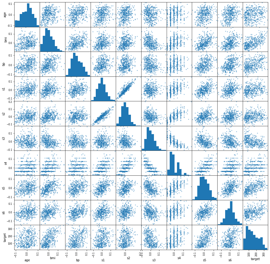
Scatter Matrix
import matplotlib.pyplot as plt

# Extract numeric data
numeric_data = data.drop(["sex"], axis=1)

# Plot scatter matrix
axes = pd.plotting.scatter_matrix(numeric_data, figsize=(15, 15))

# Fix y-axis label formatting
new_labels = [
    round(float(i.get_text()), 2) for i in axes[0, 0].get_yticklabels()
]
_ = axes[0, 0].set_yticklabels(new_labels)

Feature Correlation
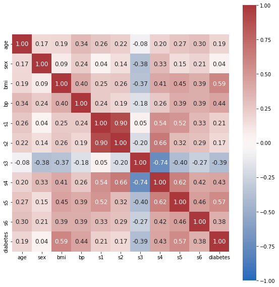
We can use seaborn’s heatmap function to inspect feature correlations.
import seaborn as sns

# Calculate correlation matrix using NumPy
correlation_matrix = np.corrcoef(data.values.T)

# Plot correlation matrix using seaborn
fig, ax = plt.subplots(figsize=(8, 8))
tick_labels = list(X.columns) + ['diabetes']
hm = sns.heatmap(
    correlation_matrix,
    ax=ax,
    cbar=True,  # Show colorbar
    cmap="vlag",  # Specify colormap
    vmin=-1,  # Min. value for colormapping
    vmax=1,  # Max. value for colormapping
    annot=True,  # Show the value of each cell
    square=True,  # Square aspect ratio in cell sizing
    fmt='.2f',  # Float formatting
    annot_kws={'size':
               12},  # Font size of the values displayed within the cells
    xticklabels=tick_labels,  # x-axis labels
    yticklabels=tick_labels)  # y-axis labels
plt.tight_layout()
plt.show()

Simple Linear Regression
Simple linear regression is a linear regression model with a single explanatory variable. bmi seems to show a discernible linear relationship with the target variable, so let’s go with that one.
Train/Test Split
from sklearn.model_selection import train_test_split

# Create a vector of the single predictor values
simple_X = X.bmi.to_numpy().reshape(len(X), 1)

# Split for simple linear regression
simple_X_train, simple_X_test, y_train, y_test = train_test_split(simple_X,
                                                                  y,
                                                                  random_state=0,
                                                                  test_size=0.2)
We now have a training dataset consisting of 353 observations and a test dataset with 89 observations.
Model Creation
from sklearn.linear_model import LinearRegression

model = LinearRegression()
_ = model.fit(simple_X_train, y_train)
Model Application
simple_y_pred = model.predict(simple_X_test)
Model Evaluation
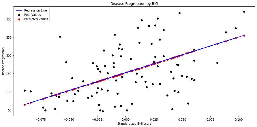
First, we’ll plot our predicted values alongside the observed values, as well as the regression line estimated by our model.
# Create figure
fig, ax = plt.subplots(figsize=(15, 7))

# Plot real values scatter plot
_ = plt.scatter(simple_X_test, y_test, color="black", label="Real Values")

# Plot predicted values scatter plot
_ = plt.scatter(simple_X_test,
                simple_y_pred,
                color="red",
                label="Predicted Values")

# Plot regression line
_ = plt.plot(simple_X_test,
             simple_y_pred,
             color="blue",
             label="Regression Line")

# Show legend
_ = plt.legend()

# Set title
title = "Disease Progression by BMI"
plt.title(title)

# Sex axis labels
ax.set_xlabel("Standardized BMI score")
_ = ax.set_ylabel("Disease Progression")

We can also use the sklearn.metrics module to calculate the MSE and coefficient of determination (\(R^2\)).
from sklearn.metrics import mean_squared_error, r2_score

mse = mean_squared_error(y_test, simple_y_pred)
r_squared = r2_score(y_train, model.predict(simple_X_train))
print(f"Coefficient: {model.coef_[0]:.2f}")
print(f"Intercept: {model.intercept_:.2f}")
print(f'Mean Squared Error: {mse:.2f}')
print(f'Coefficient of Determination: {r_squared:.2f}')
Coefficient: 981.66
Intercept: 152.29
Mean Squared Error: 4150.68
Coefficient of Determination: 0.38
Multiple Linear Regression
General notation:
Calculating the coefficient vector of the least-squares hyperplane:
Manual Implementation
While it is always best to use the standard tools Python offers, let’s be educationally paranoid for a minute and create our own implementation of ordinary least-squared (OLS) multiple linear regression.
A simplist implementation might look something like:
import numpy as np
import pandas as pd


def append_intercept(X: pd.DataFrame) -> pd.DataFrame:
    """
    Append a column of ones to the beginning of the dataset.

    Parameters
    ----------
    X : pd.DataFrame
        Observed features data

    Returns
    -------
    pd.DataFrame
        Design matrix
    """
    intercept = np.ones((len(X), 1))
    return np.hstack([intercept, X])


def estimate_coefficients(X: pd.DataFrame, y: np.ndarray) -> np.ndarray:
    """
    Returns the estimated beta hat vector.

    Parameters
    ----------
    X : pd.DataFrame
        Observed features data
    y : np.ndarray
        Target vector

    Returns
    -------
    np.ndarray
        Estimated coefficients
    """
    X = append_intercept(X)
    return np.linalg.inv(X.T @ X) @ (X.T @ y)


def calculate_predictions(X: pd.DataFrame, beta_hat: np.ndarray) -> np.ndarray:
    """
    Returns the predicted values for a test set of observations (X) using a
    vector of the estimated coefficients.

    Parameters
    ----------
    X : pd.DataFrame
        Test features data
    beta_hat : np.ndarray
        Estimated coefficients vector

    Returns
    -------
    np.ndarray
        Estimated coefficients
    """
    X = append_intercept(X)
    return X @ beta_hat
Another version, which better conforms with standard implementations in machine learning models, might look something like:
class ManualLinearRegression:
    """
    Manual implementation of an Ordinary Least Squares (OLS) linear regression
    model.
    """

    def __init__(self) -> None:
        """
        Initializes a new instance of the ManualLinearRegression model.
        """
        self.beta_hat = None

    def append_intercept(self, X: pd.DataFrame) -> pd.DataFrame:
        """
        Append a column of ones to the beginning of the dataset.

        Parameters
        ----------
        X : pd.DataFrame
            Observed features data

        Returns
        -------
        pd.DataFrame
            Design matrix
        """
        intercept = np.ones((len(X), 1))
        return np.hstack([intercept, X])

    def estimate_coefficients(
        self, X: pd.DataFrame, y: np.ndarray
    ) -> np.ndarray:
        """
        Returns the estimated beta hat vector.

        Parameters
        ----------
        X : pd.DataFrame
            Observed features data
        y : np.ndarray
            Target vector

        Returns
        -------
        np.ndarray
            Estimated coefficients
        """
        X = self.append_intercept(X)
        return np.linalg.inv(X.T @ X) @ (X.T @ y)

    def fit(self, X: pd.DataFrame, y: np.ndarray) -> None:
        """
        Calculate the estimated coefficients vector (beta hat).

        Parameters
        ----------
        X : pd.DataFrame
            Observed features data
        y : np.ndarray
            Target vector
        """
        self.beta_hat = self.estimate_coefficients(X, y)

    def predict(self, X: pd.DataFrame):
        """
        Returns the predicted values for a test set of observations (X) using a
        vector of the estimated coefficients.

        Parameters
        ----------
        X : pd.DataFrame
            Test features data
        beta_hat : np.ndarray
            Estimated coefficients vector

        Returns
        -------
        np.ndarray
            Estimated coefficients
        """
        if self.beta_hat is not None:
            X = self.append_intercept(X)
            return X @ self.beta_hat
        raise RuntimeError("Please fit the model before calling predict().")
Model Application
X_train, X_test, y_train, y_test = train_test_split(X,
                                                    y,
                                                    random_state=0,
                                                    test_size=0.2)
beta_hat = estimate_coefficients(X_train, y_train)
y_pred_manual = calculate_predictions(X_test, beta_hat)
or:
manual_model = ManualLinearRegression()
manual_model.fit(X_train, y_train)
y_pred_manual = manual_model.predict(X_test)
Model Evaluation
\(R^2\)
Calculate the residual sum of squares (\(RSS\)):
General notation
Matrix notation
ss_residual = np.sum((y_train - manual_model.predict(X_train))**2)
ss_residual
965359.4331583097
Calculate the total sum of squares (\(TSS\)):
ss_total = np.sum((y_train - y_train.mean())**2)
ss_total
2164136.266288952
Calculate \(R^2\):
r2_score_manual = 1 - ss_residual / ss_total
r2_score_manual
0.5539285357415583
Compare with sklearn’s built-in r2_score function:
r2_score(y_true=y_train, y_pred=manual_model.predict(X_train))
0.5539285357415583
Mean Squared Error
Manual \(MSE\) calculation:
mse_manual = np.mean((y_train - manual_model.predict(X_train))**2)
mse_manual
2734.7292724031436
Or using sklearn:
mean_squared_error(y_train, manual_model.predict(X_train))
2734.7292724031436
Multiple Linear Regression using sklearn
Model Creation
multiple_model = LinearRegression()
_ = multiple_model.fit(X_train, y_train)
Model Application
y_pred_all = multiple_model.predict(X_test)
Model Evaluation
mse_all = mean_squared_error(y_train, multiple_model.predict(X_train))
r2_score_all = r2_score(y_train, multiple_model.predict(X_train))
betas_all_repr = [beta.round(2) for beta in multiple_model.coef_.flatten()]

print(f"Coefficient: {betas_all_repr}")
print(f'Mean Squared Error: {mse_all:.2f}')
Coefficient: [-35.56, -243.17, 562.75, 305.47, -662.79, 324.28, 24.78, 170.33, 731.68, 43.03]
Mean Squared Error: 2734.73


