Exercise IV: Logistic Regression
In statistics, the logistic model (or logit model) is used to model the probability of a certain class or event existing such as pass/fail, win/lose, alive/dead or healthy/sick. This can be extended to model several classes of events such as determining whether an image contains a cat, dog, lion, etc. Each object being detected in the image would be assigned a probability between 0 and 1, with a sum of one. Wikipedia
In this exercise we will reproduce the bank defaults example used in chapter IV of the ISLR, as adapted from the ISLR-python repository.
Setup
import warnings
warnings.simplefilter("ignore")
import pandas as pd

URL = "https://github.com/JWarmenhoven/ISLR-python/raw/master/Notebooks/Data/Default.xlsx"
df = pd.read_excel(URL, index_col=0, true_values=["Yes"], false_values=["No"])
def color_booleans(value: bool) -> str:
    color = "green" if value else "red"
    return f"color: {color}"

BOOLEAN_COLUMNS = ["default", "student"]

df.sample(15).style.text_gradient(cmap="Blues").applymap(color_booleans, subset=BOOLEAN_COLUMNS)
| default | student | balance | income | |
|---|---|---|---|---|
| 1097 | False | True | 1461.833249 | 19252.237291 |
| 2192 | False | True | 1295.029713 | 21717.469549 |
| 1393 | False | False | 468.412124 | 22943.125687 |
| 7933 | False | True | 1273.488513 | 17105.867047 |
| 7366 | False | False | 149.822550 | 33948.866290 |
| 280 | False | False | 369.221942 | 47835.091045 |
| 9352 | False | False | 0.000000 | 62160.286220 |
| 5618 | False | False | 1267.001444 | 32752.193741 |
| 5537 | False | False | 514.849025 | 37656.847872 |
| 1100 | False | False | 1516.551152 | 39368.141873 |
| 4184 | False | False | 202.070433 | 28814.175306 |
| 6557 | False | False | 1135.187984 | 47075.032300 |
| 4728 | False | True | 649.360117 | 10524.326101 |
| 5343 | False | False | 1277.123098 | 42472.908266 |
| 7496 | False | False | 717.667390 | 27956.273520 |
Feature Scaling
import numpy as np
from sklearn.preprocessing import StandardScaler

numeric_features = df.select_dtypes(np.float)
scaler = StandardScaler()
df.loc[:, numeric_features.columns] = scaler.fit_transform(df.loc[:, numeric_features.columns])
Raw inspection
df.info()
<class 'pandas.core.frame.DataFrame'>
Int64Index: 10000 entries, 1 to 10000
Data columns (total 4 columns):
 #   Column   Non-Null Count  Dtype
---  ------   --------------  -----
 0   default  10000 non-null  bool
 1   student  10000 non-null  bool
 2   balance  10000 non-null  float64
 3   income   10000 non-null  float64
dtypes: bool(2), float64(2)
memory usage: 253.9 KB
pd.set_option('float_format', '{:g}'.format)
df.describe()
| balance | income | |
|---|---|---|
| count | 10000 | 10000 |
| mean | -1.25056e-16 | -1.93623e-16 |
| std | 1.00005 | 1.00005 |
| min | -1.72708 | -2.45539 |
| 25% | -0.731136 | -0.913058 |
| 50% | -0.0242674 | 0.0776593 |
| 75% | 0.684184 | 0.771653 |
| max | 3.76056 | 3.0022 |
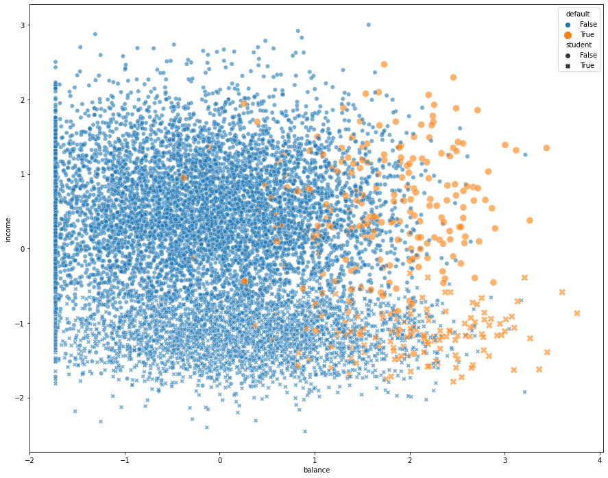
Scatter plot
import matplotlib.pyplot as plt
import seaborn as sns

fix, ax = plt.subplots(figsize=(15, 12))
_ = sns.scatterplot(x="balance",
                    y="income",
                    hue="default",
                    style="student",
                    size="default",
                    sizes={
                        True: 100,
                        False: 40
                    },
                    alpha=0.6,
                    ax=ax,
                    data=df)
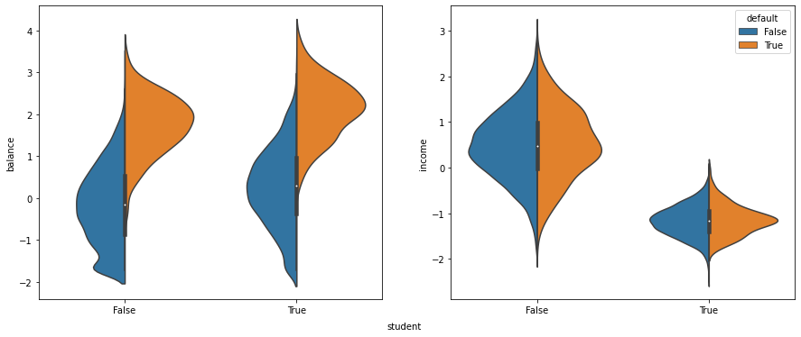
Violin plot
# Create a new figure with two horizontal subplots
fig, ax = plt.subplots(ncols=2, figsize=(15, 6))

# Plot balance
sns.violinplot(x="student", y="balance", hue="default", split=True, legend=False, ax=ax[0], data=df)
ax[0].get_legend().remove()
ax[0].set_xlabel('')

# Plot income
sns.violinplot(x="student", y="income", hue="default", split=True, ax=ax[1], data=df)
ax[1].set_xlabel('')

# Add common label
_ = fig.text(0.5, 0.05, "student", ha='center')
Train/Test Split
from sklearn.model_selection import train_test_split

FEATURE_NAMES = ["balance", "income", "student"]
TARGET_NAME = "default"
X = df[FEATURE_NAMES]
y = df[TARGET_NAME].values

X_train, X_test, y_train, y_test = train_test_split(X,
                                                    y,
                                                    random_state=0,
                                                    test_size=0.2)
Model Creation
sklearn
from sklearn.linear_model import LogisticRegression

sk_model = LogisticRegression(random_state=0, penalty="none", solver="newton-cg")
_ = sk_model.fit(X_train, y_train)
statsmodels
import statsmodels.api as sm

# statsmodels requires booelean values to be converted to integers.
df["student"] = df["student"].astype(int)
df["default"] = df["default"].astype(int)

# R-style model formulation.
sm_model = sm.Logit.from_formula('default ~ balance + income + student', data=df)
Model Application
sklearn
We can predict the probability estimates of each target class (in our case True or False) using the LogisticRegression class’s predict_proba() method:
default_probability = sk_model.predict_proba(X_test)
Or, we could directly return the predictions based on the maximal probabilities:
predictions = sk_model.predict(X_test)

# Manually returning the index of the maximal value
predictions_manual = default_probability.argmax(axis=1)

np.array_equal(predictions, predictions_manual)
True
statsmodels
sm_estimation = sm_model.fit()
Optimization terminated successfully.
         Current function value: 0.078577
         Iterations 10
Model Evaluation
sklearn
print(f"Intercept: {sk_model.intercept_}")
print(f"Coefficients: {sk_model.coef_}")
Intercept: [-5.93187127]
Coefficients: [[ 2.72019068 -0.02263331 -0.61746372]]
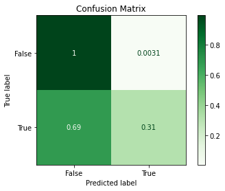
Confusion Matrix
Calculation
from sklearn.metrics import confusion_matrix

confusion_matrix_ = confusion_matrix(y_test, predictions)
print(confusion_matrix_)
[[1920    6]
 [  51   23]]
Visualization
from sklearn.metrics import plot_confusion_matrix

disp = plot_confusion_matrix(sk_model,
                             X_test,
                             y_test,
                             cmap=plt.cm.Greens,
                             normalize="true")
_ = disp.ax_.set_title(f"Confusion Matrix")
Classification Report
from sklearn.metrics import classification_report

report = classification_report(y_test, predictions)
print(report)
              precision    recall  f1-score   support

       False       0.97      1.00      0.99      1926
        True       0.79      0.31      0.45        74

    accuracy                           0.97      2000
   macro avg       0.88      0.65      0.72      2000
weighted avg       0.97      0.97      0.97      2000
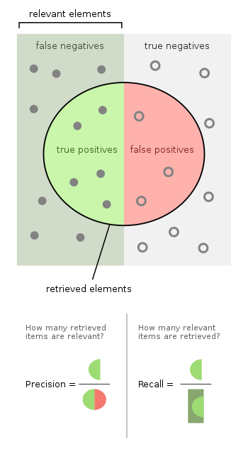
Precision

true_positive = confusion_matrix_[1, 1]
false_positive = confusion_matrix_[0, 1]

true_positive / (true_positive + false_positive)
0.7931034482758621
Recall (Sensitivity)

false_negative = confusion_matrix_[1, 0]

true_positive / (true_positive + false_negative)
0.3108108108108108
Specificity

true_negative = confusion_matrix_[0, 0]

true_negative / (true_negative + false_positive)
0.9968847352024922
Accuracy Score
from sklearn.metrics import accuracy_score

accuracy_score(y_test, predictions)
0.9715
or:
true_predictions = confusion_matrix_[0, 0] + confusion_matrix_[1, 1]
true_predictions / len(X_test)
0.9715
statsmodels
Confusion Matrix
prediction_table = sm_estimation.pred_table()
prediction_table
array([[9627.,   40.],
       [ 228.,  105.]])
row_sums = prediction_table.sum(axis=1, keepdims=True)
prediction_table / row_sums
array([[0.99586221, 0.00413779],
       [0.68468468, 0.31531532]])
Regression Report
sm_estimation.summary()
| Dep. Variable: | default | No. Observations: | 10000 |
|---|---|---|---|
| Model: | Logit | Df Residuals: | 9996 |
| Method: | MLE | Df Model: | 3 |
| Date: | Wed, 15 Dec 2021 | Pseudo R-squ.: | 0.4619 |
| Time: | 07:44:26 | Log-Likelihood: | -785.77 |
| converged: | True | LL-Null: | -1460.3 |
| Covariance Type: | nonrobust | LLR p-value: | 3.257e-292 |
| coef | std err | z | P>|z| | [0.025 | 0.975] | |
|---|---|---|---|---|---|---|
| Intercept | -5.9752 | 0.194 | -30.849 | 0.000 | -6.355 | -5.596 |
| balance | 2.7747 | 0.112 | 24.737 | 0.000 | 2.555 | 2.995 |
| income | 0.0405 | 0.109 | 0.370 | 0.712 | -0.174 | 0.255 |
| student | -0.6468 | 0.236 | -2.738 | 0.006 | -1.110 | -0.184 |
Possibly complete quasi-separation: A fraction 0.15 of observations can be
perfectly predicted. This might indicate that there is complete
quasi-separation. In this case some parameters will not be identified.