Exercise V: Regularization
This exercise is an adaptation of lab 2 from the ISLR, in which the salary of baseball players is predicted on the basis of various statistics associated with performance in the previous year.
Set up
import pandas as pd

URL = "https://raw.githubusercontent.com/JWarmenhoven/ISLR-python/master/Notebooks/Data/Hitters.csv"
data = pd.read_csv(URL, index_col=0)
General Inspection and Preprocessing
data
| AtBat | Hits | HmRun | Runs | RBI | Walks | Years | CAtBat | CHits | CHmRun | CRuns | CRBI | CWalks | League | Division | PutOuts | Assists | Errors | Salary | NewLeague | |
|---|---|---|---|---|---|---|---|---|---|---|---|---|---|---|---|---|---|---|---|---|
| -Andy Allanson | 293 | 66 | 1 | 30 | 29 | 14 | 1 | 293 | 66 | 1 | 30 | 29 | 14 | A | E | 446 | 33 | 20 | NaN | A |
| -Alan Ashby | 315 | 81 | 7 | 24 | 38 | 39 | 14 | 3449 | 835 | 69 | 321 | 414 | 375 | N | W | 632 | 43 | 10 | 475.0 | N |
| -Alvin Davis | 479 | 130 | 18 | 66 | 72 | 76 | 3 | 1624 | 457 | 63 | 224 | 266 | 263 | A | W | 880 | 82 | 14 | 480.0 | A |
| -Andre Dawson | 496 | 141 | 20 | 65 | 78 | 37 | 11 | 5628 | 1575 | 225 | 828 | 838 | 354 | N | E | 200 | 11 | 3 | 500.0 | N |
| -Andres Galarraga | 321 | 87 | 10 | 39 | 42 | 30 | 2 | 396 | 101 | 12 | 48 | 46 | 33 | N | E | 805 | 40 | 4 | 91.5 | N |
| ... | ... | ... | ... | ... | ... | ... | ... | ... | ... | ... | ... | ... | ... | ... | ... | ... | ... | ... | ... | ... |
| -Willie McGee | 497 | 127 | 7 | 65 | 48 | 37 | 5 | 2703 | 806 | 32 | 379 | 311 | 138 | N | E | 325 | 9 | 3 | 700.0 | N |
| -Willie Randolph | 492 | 136 | 5 | 76 | 50 | 94 | 12 | 5511 | 1511 | 39 | 897 | 451 | 875 | A | E | 313 | 381 | 20 | 875.0 | A |
| -Wayne Tolleson | 475 | 126 | 3 | 61 | 43 | 52 | 6 | 1700 | 433 | 7 | 217 | 93 | 146 | A | W | 37 | 113 | 7 | 385.0 | A |
| -Willie Upshaw | 573 | 144 | 9 | 85 | 60 | 78 | 8 | 3198 | 857 | 97 | 470 | 420 | 332 | A | E | 1314 | 131 | 12 | 960.0 | A |
| -Willie Wilson | 631 | 170 | 9 | 77 | 44 | 31 | 11 | 4908 | 1457 | 30 | 775 | 357 | 249 | A | W | 408 | 4 | 3 | 1000.0 | A |
322 rows × 20 columns
Well, it looks like a dataset.
Let’s probe a little deeper:
data.info()
<class 'pandas.core.frame.DataFrame'>
Index: 322 entries, -Andy Allanson to -Willie Wilson
Data columns (total 20 columns):
 #   Column     Non-Null Count  Dtype
---  ------     --------------  -----
 0   AtBat      322 non-null    int64
 1   Hits       322 non-null    int64
 2   HmRun      322 non-null    int64
 3   Runs       322 non-null    int64
 4   RBI        322 non-null    int64
 5   Walks      322 non-null    int64
 6   Years      322 non-null    int64
 7   CAtBat     322 non-null    int64
 8   CHits      322 non-null    int64
 9   CHmRun     322 non-null    int64
 10  CRuns      322 non-null    int64
 11  CRBI       322 non-null    int64
 12  CWalks     322 non-null    int64
 13  League     322 non-null    object
 14  Division   322 non-null    object
 15  PutOuts    322 non-null    int64
 16  Assists    322 non-null    int64
 17  Errors     322 non-null    int64
 18  Salary     263 non-null    float64
 19  NewLeague  322 non-null    object
dtypes: float64(1), int64(16), object(3)
memory usage: 52.8+ KB
Calling info() reveals that most (16/19) columns contain integers, except for Salary which is a float and League, NewLeague, and Division which are object (categorical). Even more importantly, it shows that Salary contains missing observations. Because Salary is our target variable, we don’t really have any use for these observations and would be better off simply dropping them from our dataset:
data.dropna(subset=["Salary"], inplace=True)
Done.
Next, we might give describe() a quick look:
pd.set_option('float_format', '{:.4g}'.format)
data.describe()
| AtBat | Hits | HmRun | Runs | RBI | Walks | Years | CAtBat | CHits | CHmRun | CRuns | CRBI | CWalks | PutOuts | Assists | Errors | Salary | |
|---|---|---|---|---|---|---|---|---|---|---|---|---|---|---|---|---|---|
| count | 263 | 263 | 263 | 263 | 263 | 263 | 263 | 263 | 263 | 263 | 263 | 263 | 263 | 263 | 263 | 263 | 263 |
| mean | 403.6 | 107.8 | 11.62 | 54.75 | 51.49 | 41.11 | 7.312 | 2658 | 722.2 | 69.24 | 361.2 | 330.4 | 260.3 | 290.7 | 118.8 | 8.593 | 535.9 |
| std | 147.3 | 45.13 | 8.757 | 25.54 | 25.88 | 21.72 | 4.794 | 2287 | 648.2 | 82.2 | 331.2 | 323.4 | 264.1 | 279.9 | 145.1 | 6.607 | 451.1 |
| min | 19 | 1 | 0 | 0 | 0 | 0 | 1 | 19 | 4 | 0 | 2 | 3 | 1 | 0 | 0 | 0 | 67.5 |
| 25% | 282.5 | 71.5 | 5 | 33.5 | 30 | 23 | 4 | 842.5 | 212 | 15 | 105.5 | 95 | 71 | 113.5 | 8 | 3 | 190 |
| 50% | 413 | 103 | 9 | 52 | 47 | 37 | 6 | 1931 | 516 | 40 | 250 | 230 | 174 | 224 | 45 | 7 | 425 |
| 75% | 526 | 141.5 | 18 | 73 | 71 | 57 | 10 | 3890 | 1054 | 92.5 | 497.5 | 424.5 | 328.5 | 322.5 | 192 | 13 | 750 |
| max | 687 | 238 | 40 | 130 | 121 | 105 | 24 | 1.405e+04 | 4256 | 548 | 2165 | 1659 | 1566 | 1377 | 492 | 32 | 2460 |
Scaling
I seems like there’s fairly large variabiliy in scale between the different features, and in any case regularization requires some form of standardization.
First, let’s differntiate the features matrix (X) from the target vector (y):
target_name = "Salary"

X = data.drop(columns=[target_name])
y = data[target_name].copy()
Only numeric columns should be standardized, so let’s also be sure to distinguish those from the categoricals:
numeric_features = X.select_dtypes([int, float])
And we’re all set:
from sklearn.preprocessing import StandardScaler

scaler = StandardScaler()
X.loc[:, numeric_features.columns] = scaler.fit_transform(
    X.loc[:, numeric_features.columns])
X
| AtBat | Hits | HmRun | Runs | RBI | Walks | Years | CAtBat | CHits | CHmRun | CRuns | CRBI | CWalks | League | Division | PutOuts | Assists | Errors | NewLeague | |
|---|---|---|---|---|---|---|---|---|---|---|---|---|---|---|---|---|---|---|---|
| -Alan Ashby | -0.6029 | -0.5957 | -0.5286 | -1.206 | -0.5221 | -0.09753 | 1.398 | 0.3468 | 0.1744 | -0.00292 | -0.1217 | 0.259 | 0.4353 | N | W | 1.221 | -0.5232 | 0.2134 | N |
| -Alvin Davis | 0.5125 | 0.4923 | 0.73 | 0.4415 | 0.7941 | 1.609 | -0.9012 | -0.4529 | -0.4099 | -0.07605 | -0.4151 | -0.1996 | 0.01037 | A | W | 2.109 | -0.2539 | 0.82 | A |
| -Andre Dawson | 0.6282 | 0.7365 | 0.9588 | 0.4023 | 1.026 | -0.1898 | 0.7709 | 1.302 | 1.318 | 1.899 | 1.412 | 1.573 | 0.3557 | N | E | -0.3247 | -0.7442 | -0.8482 | N |
| -Andres Galarraga | -0.5621 | -0.4625 | -0.1853 | -0.6177 | -0.3672 | -0.5127 | -1.11 | -0.9909 | -0.9602 | -0.6977 | -0.9475 | -0.8812 | -0.8623 | N | E | 1.841 | -0.5439 | -0.6966 | N |
| -Alfredo Griffin | 1.295 | 1.358 | -0.8718 | 0.7553 | -0.01884 | -0.2821 | 0.7709 | 0.767 | 0.635 | -0.6124 | 0.4228 | 0.01729 | -0.2514 | A | W | -0.03118 | 2.087 | 2.488 | A |
| ... | ... | ... | ... | ... | ... | ... | ... | ... | ... | ... | ... | ... | ... | ... | ... | ... | ... | ... | ... |
| -Willie McGee | 0.635 | 0.4257 | -0.5286 | 0.4023 | -0.135 | -0.1898 | -0.4832 | 0.01992 | 0.1295 | -0.4539 | 0.05378 | -0.06016 | -0.4639 | N | E | 0.1227 | -0.758 | -0.8482 | N |
| -Willie Randolph | 0.601 | 0.6255 | -0.7574 | 0.8338 | -0.05755 | 2.44 | 0.9799 | 1.25 | 1.219 | -0.3686 | 1.621 | 0.3736 | 2.332 | A | E | 0.07977 | 1.811 | 1.73 | A |
| -Wayne Tolleson | 0.4853 | 0.4034 | -0.9862 | 0.2454 | -0.3285 | 0.5022 | -0.2742 | -0.4196 | -0.447 | -0.7586 | -0.4363 | -0.7356 | -0.4336 | A | W | -0.9081 | -0.03978 | -0.2416 | A |
| -Willie Upshaw | 1.152 | 0.8031 | -0.2997 | 1.187 | 0.3295 | 1.702 | 0.1438 | 0.2368 | 0.2084 | 0.3384 | 0.3291 | 0.2776 | 0.2722 | A | E | 3.662 | 0.08452 | 0.5167 | A |
| -Willie Wilson | 1.546 | 1.38 | -0.2997 | 0.873 | -0.2898 | -0.4666 | 0.7709 | 0.9861 | 1.136 | -0.4783 | 1.252 | 0.08236 | -0.04275 | A | W | 0.4198 | -0.7925 | -0.8482 | A |
263 rows × 19 columns
X.describe()
| AtBat | Hits | HmRun | Runs | RBI | Walks | Years | CAtBat | CHits | CHmRun | CRuns | CRBI | CWalks | PutOuts | Assists | Errors | |
|---|---|---|---|---|---|---|---|---|---|---|---|---|---|---|---|---|
| count | 263 | 263 | 263 | 263 | 263 | 263 | 263 | 263 | 263 | 263 | 263 | 263 | 263 | 263 | 263 | 263 |
| mean | 1.013e-17 | 5.741e-17 | 3.377e-17 | -5.066e-17 | 1.216e-16 | 1.689e-18 | -5.403e-17 | 6.079e-17 | 6.754e-17 | 5.403e-17 | 3.377e-17 | 4.053e-17 | 1.081e-16 | 7.43e-17 | 0 | 1.047e-16 |
| std | 1.002 | 1.002 | 1.002 | 1.002 | 1.002 | 1.002 | 1.002 | 1.002 | 1.002 | 1.002 | 1.002 | 1.002 | 1.002 | 1.002 | 1.002 | 1.002 |
| min | -2.616 | -2.372 | -1.329 | -2.148 | -1.993 | -1.897 | -1.319 | -1.156 | -1.11 | -0.844 | -1.087 | -1.014 | -0.9837 | -1.04 | -0.8201 | -1.303 |
| 25% | -0.8239 | -0.8066 | -0.7574 | -0.8334 | -0.8317 | -0.8356 | -0.6922 | -0.7953 | -0.7886 | -0.6611 | -0.7736 | -0.7294 | -0.7181 | -0.6343 | -0.7649 | -0.8482 |
| 50% | 0.06364 | -0.1072 | -0.2997 | -0.1077 | -0.1737 | -0.1898 | -0.2742 | -0.3183 | -0.3187 | -0.3564 | -0.3365 | -0.3111 | -0.3273 | -0.2388 | -0.5094 | -0.2416 |
| 75% | 0.8322 | 0.7476 | 0.73 | 0.7161 | 0.7554 | 0.7329 | 0.5619 | 0.5402 | 0.5129 | 0.2835 | 0.4123 | 0.2915 | 0.2589 | 0.1138 | 0.5058 | 0.6683 |
| max | 1.927 | 2.89 | 3.247 | 2.952 | 2.691 | 2.947 | 3.488 | 4.993 | 5.462 | 5.836 | 5.457 | 4.116 | 4.954 | 3.888 | 2.578 | 3.55 |
Warning
Try to consider the way in which standardization was applied. Can you think of anything that could pose a problem in following steps?
Solution
Applying standardization prior to the train-test split results in information (mean and standard deviation) from the test set “leaking” into the training set, and therefore should be avoided! The correct procedure is to apply standardization separately after splitting the data.
Dummy Encoding
To view the different values each categorical variable holds:
for feature in X.select_dtypes(object):
    print(feature.ljust(10), X[feature].unique())
League     ['N' 'A']
Division   ['W' 'E']
NewLeague  ['N' 'A']
And to “dummy encode” it is as simple as:
X = pd.get_dummies(X, drop_first=True)
X.sample(20).select_dtypes(include=["uint8"]).style.background_gradient()
| League_N | Division_W | NewLeague_N | |
|---|---|---|---|
| -Ken Landreaux | 1 | 1 | 1 |
| -Ron Hassey | 0 | 0 | 0 |
| -Shawon Dunston | 1 | 0 | 1 |
| -Chris Bando | 0 | 0 | 0 |
| -Don Mattingly | 0 | 0 | 0 |
| -Ken Phelps | 0 | 1 | 0 |
| -Gary Carter | 1 | 0 | 1 |
| -Al Newman | 1 | 0 | 0 |
| -Rick Dempsey | 0 | 0 | 0 |
| -Wally Joyner | 0 | 1 | 0 |
| -Kevin Bass | 1 | 1 | 1 |
| -Leon Durham | 1 | 0 | 1 |
| -Jesse Barfield | 0 | 0 | 0 |
| -Brian Downing | 0 | 1 | 0 |
| -Tom Brunansky | 0 | 1 | 0 |
| -Terry Kennedy | 1 | 1 | 0 |
| -Jody Davis | 1 | 0 | 1 |
| -Dwight Evans | 0 | 0 | 0 |
| -Argenis Salazar | 0 | 1 | 0 |
| -Ted Simmons | 1 | 1 | 1 |
Model Creation
In the previous linear regression exercise we used sklearn’s LinearRegression class along with the train_test_split() function to model the relationship between the features and the target variable and evaluate it’s performance in predicting the target variable for an out-of-sample collection of observations. In this exercise, we will use LassoCV and RidgeCV to introduce the \(\ell_1\) and \(\ell_2\) penalties as part of our fitting process and regularize the coefficients of our predictors. In addition, cross-validation will also be taken care of automatically.
For the sake of uniformity we’ll use the same list of regularization parameter values:
import numpy as np

alphas = np.linspace(0.01, 100, 200)
Lasso (\(\ell_1\))
from sklearn.linear_model import LassoCV

lasso_model = LassoCV(alphas=alphas, max_iter=10000)
_ = lasso_model.fit(X, y)
Ridge (\(\ell_2\))
from sklearn.linear_model import RidgeCV

ridge_model = RidgeCV(alphas=alphas, store_cv_values=True)
_ = ridge_model.fit(X, y)
Note
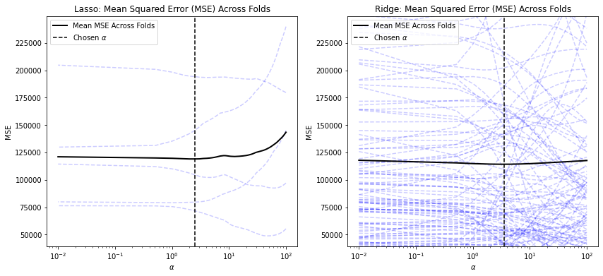
By default, LassoCV will use 5-fold cross-validation with \(R^2\) as the scoring method and RidgeCV will use Generalized Cross-Validation, which is a form of efficient Leave-One-Out cross-validation, with negative mean squared error.
To change the splitting strategy, set the cv keyword argument to the number of folds you’d like to use, to specify scoring and other search parameters see the GridSearchCV class.
Model Application
To calculate the predicted salary of each player using the model:
Lasso (\(\ell_1\))
lasso_predictions = lasso_model.predict(X)
Ridge (\(\ell_2\))
ridge_predictions = ridge_model.predict(X)
Model Evaluation
import matplotlib.pyplot as plt


def plot_predictions(y: pd.Series, predictions: pd.Series, ax: plt.Axes):
    ax.scatter(y, predictions, color="black")
    ax.plot(y, y, color="red")
    ax.set_xlabel("Real Values")
    ax.set_ylabel("Predicted Values")


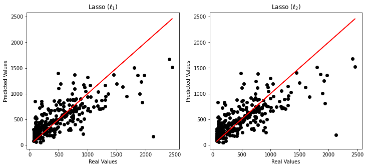
fig, ax = plt.subplots(ncols=2, figsize=(12, 5))
plot_predictions(y, lasso_predictions, ax[0])
ax[0].set_title(r"Lasso ($\ell_1$)")
plot_predictions(y, ridge_predictions, ax[1])
_ = ax[1].set_title(r"Lasso ($\ell_2$)")

Alpha
Lasso (\(\ell_1\))
lasso_model.alpha_
2.522311557788944
Ridge (\(\ell_2\))
ridge_model.alpha_
3.527236180904522
Coefficients
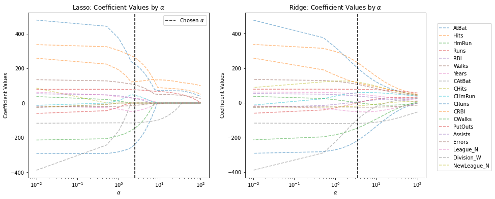
coefficients_dict = {"Lasso": lasso_model.coef_, "Ridge": ridge_model.coef_}
coefficients = pd.DataFrame(coefficients_dict, index=X.columns)
coefficients.T
| AtBat | Hits | HmRun | Runs | RBI | Walks | Years | CAtBat | CHits | CHmRun | CRuns | CRBI | CWalks | PutOuts | Assists | Errors | League_N | Division_W | NewLeague_N | |
|---|---|---|---|---|---|---|---|---|---|---|---|---|---|---|---|---|---|---|---|
| Lasso | -237.2 | 261.6 | 0 | -0 | 0 | 104.8 | -46.64 | -0 | 0 | 44.29 | 224.5 | 123.9 | -144.8 | 76.81 | 26.48 | -13.56 | 27.04 | -114.1 | 0 |
| Ridge | -216.4 | 230.7 | 0.9447 | 0.7865 | 6.002 | 106.3 | -51.34 | -94.18 | 119.4 | 58.18 | 199.9 | 114.5 | -144.5 | 77.68 | 39.18 | -24.86 | 50.73 | -118.6 | -18.02 |
from sklearn.linear_model import Lasso, Ridge


coef_fig, coef_ax = plt.subplots(ncols=2, figsize=(14, 6))

#########
# Lasso #
#########

simple_lasso = Lasso(max_iter=10_000)
lasso_coefficient_values = []
lasso_alphas = lasso_model.alphas_[::-1]

for alpha in lasso_alphas:
    simple_lasso.set_params(alpha=alpha)
    simple_lasso.fit(X, y)
    lasso_coefficient_values.append(simple_lasso.coef_)

# Coefficient values by alpha
coef_ax[0].semilogx(lasso_alphas, lasso_coefficient_values, linestyle="dashed", alpha=0.5)

# Chosen alpha
coef_ax[0].axvline(lasso_model.alpha_,
                  linestyle='--',
                  color="black",
                  label=r"Chosen $\alpha$")
coef_ax[0].legend()
coef_ax[0].set_xlabel(r'$\alpha$')
coef_ax[0].set_ylabel("Coefficient Values")
coef_ax[0].set_title(r"Lasso: Coefficient Values by $\alpha$")

#########
# Ridge #
#########

simple_ridge = Ridge()
ridge_coefficient_values = []
ridge_alphas = ridge_model.alphas[::-1]

for alpha in ridge_alphas:
    simple_ridge.set_params(alpha=alpha)
    simple_ridge.fit(X, y)
    ridge_coefficient_values.append(simple_ridge.coef_)


# Coefficient values by alpha
coef_ax[1].semilogx(ridge_alphas,
                   ridge_coefficient_values,
                   linestyle="dashed",
                   alpha=0.5)
# Chosen alpha
coef_ax[1].axvline(ridge_model.alpha_,
                  linestyle='--',
                  color="black",
                  label=r"Chosen $\alpha$")
coef_ax[1].legend(X.columns, loc="upper left", bbox_to_anchor=(1.05, 0.95))
coef_ax[1].set_xlabel(r'$\alpha$')
coef_ax[1].set_ylabel("Coefficient Values")
_ = coef_ax[1].set_title(r"Ridge: Coefficient Values by $\alpha$")

Mean Squared Error (MSE)
mse_fig, mse_ax = plt.subplots(ncols=2, figsize=(14, 6))

#########
# Lasso #
#########

lasso_alphas = lasso_model.alphas_
lasso_mse = lasso_model.mse_path_

# Cross-validation MSEs
mse_ax[0].semilogx(lasso_alphas,
                   lasso_mse,
                   linestyle="dashed",
                   color="blue",
                   alpha=0.2)

# Mean MSE
mse_ax[0].plot(lasso_alphas,
               lasso_mse.mean(axis=-1),
               color="black",
               label="Mean MSE Across Folds",
               linewidth=2)
# Chosen alpha
mse_ax[0].axvline(lasso_model.alpha_,
                  linestyle='--',
                  color="black",
                  label=r"Chosen $\alpha$")
mse_ax[0].legend()
mse_ax[0].set_xlabel(r'$\alpha$')
mse_ax[0].set_ylabel("MSE")
mse_ax[0].set_title("Lasso: Mean Squared Error (MSE) Across Folds")

#########
# Ridge #
#########

ridge_alphas = ridge_model.alphas
ridge_mse = ridge_model.cv_values_.T

# Cross-validation MSEs
mse_ax[1].semilogx(ridge_alphas,
                   ridge_mse,
                   linestyle="dashed",
                   color="blue",
                   alpha=0.2)
# Mean MSE
mse_ax[1].plot(ridge_alphas,
               ridge_mse.mean(axis=-1),
               color="black",
               label="Mean MSE Across Folds",
               linewidth=2)
# Chosen alpha
mse_ax[1].axvline(ridge_model.alpha_,
                  linestyle='--',
                  color="black",
                  label=r"Chosen $\alpha$")
mse_ax[1].legend()
mse_ax[1].set_xlabel(r'$\alpha$')
mse_ax[1].set_ylabel("MSE")
mse_ax[1].ticklabel_format(style="plain", axis="y")
mse_ax[1].set_ylim(mse_ax[0].get_ylim())
_ = mse_ax[1].set_title("Ridge: Mean Squared Error (MSE) Across Folds")

\(R^2\)
To calculate in-sample \(R^2\) score for each model:
Lasso (\(\ell_1\))
lasso_model.score(X, y)
0.5342574616741457
Ridge (\(\ell_2\))
ridge_model.score(X, y)
0.5364706351171298
Note that calculating in-sample \(R^2\) scores will result in underestimating prediction error.
Note
For a more generalized solution for parameter tuning, see sklearn’s GridSearchCV.

